
At the end of my last Power BI performance blog post, I mentioned that I wanted to get into the details of optimizations that can be done on your DAX code to ensure that you are getting the best performance that you can from Power BI. In this blog post, we hope to help you understand how the VertiPaq engine works a bit below surface level, which can help you optimize your DAX code. While doing this, we are going to emphasize a DAX performance maxim: Filter columns, not tables. Before we go there, let’s review how Power BI processes your DAX code.

In Part I of my series, I talked about how the VertiPaq engine in SSAS Tabular and Power BI use highly-efficient compression algorithms to greatly reduce the amount of storage space needed to store your data. You want as much of it as possible stored in RAM and/or the CPU caches. That’s great that we can compress the data down so much, but what happens when we need to read all that data? Do we have to re-expand it all again to read it? This doesn’t seem like it would be a good idea. If Power BI worked so hard to compress all the data, are we just reversing that when we have to read it?
How Does Power BI Read This Compressed Data?
To better understand what’s going on, it’s important to know that your DAX code is being processed by two different engines, the formula engine and the storage engine. The formula engine processes your DAX code, understands it, and makes a plan for how to retrieve the data needed to execute your code. It then uses this plan to make a series of queries with the storage engine to retrieve the data, evaluate the results, and return the information needed to satisfy your DAX code.
The formula engine has to be very sophisticated to both interpret your DAX code and to put together a plan on what data can be retrieved. As a result, it is single threaded. No matter how many CPUs or Cores you have, the formula engine will only run one step at a time. It also only understands data that has been decompressed or materialized, so when it needs to read data you will pay a price in performance to have the data expanded.
The storage engine, on the other hand, is built for speed and can run with multiple threads. This focus on speed means that it’s not as sophisticated as the formula engine, but it can process compressed data without having to expand it first. The storage engine takes requests for data from the formula engine and retrieves it from the compressed data.
As a general performance rule then, the more work you can push to the fast, multi-threaded storage engine the better because its faster. Bless its heart though (as they say in the South), it just can’t handle complex operations. Therefore, optimizing DAX code can sometimes mean balancing what has to be retrieved and materialized for consumption by the formula engine versus what can be processed by the storage engine.
Filter Columns, Not Tables
I have a simple data model that contains weather data collected from weather stations across the United States from 1938 to the present. This weather data is a daily measurement of the minimum, maximum, and average temperature over a 24-hour period. The data comes from over 17,000 weather stations, so the fact table is over 430 million rows. I have the model set up with a fact table, date dimension table, and a station dimension table that contains information about the station’s location, elevation, city, and state. The model is a very simple star schema as shown below:

So, first I want to know how many temperature readings there are in my entire collection grouped by state. The DAX to do this is straightforward, so I will test it in DAX Studio and see what the performance is. DAX Studio is an open-source DAX editor and performance tool that I use almost daily. You can find the latest version here.
DAX Studio lets me execute queries and capture the query plans produced, as well as execution statistics. The details of how to do this is outside the scope of this blog, but if you look at the screenshot below, you can see that I defined a measure, then called it from a DAX statement. DAX Studio breaks down the query into formula engine and storage engine queries and provides details on their execution.

The DAX I used to get my temperature readings by state was the following:
DEFINE
MEASURE Fact[PositiveValues] = CALCULATE(DISTINCTCOUNT(‘Fact'[value]))
EVALUATE
CALCULATETABLE(SUMMARIZECOLUMNS(Stations[State], “# of Values”, [PositiveValues]))
If I look at the server timings data captured by DAX Studio, even without knowing too much about the internals of the storage queries, you can tell that this was fast.

The total amount of time it took to run was 293 milliseconds, and it took just one Storage Engine query to return 52 rows (50 states plus DC & US Minor Outlying Islands) of data. The data materialized was somewhere around a KB. That’s smokin’ fast!
Now, say I want to only count the number of daily minimum values that are greater than zero. Let’s throw some DAX together and take a look at how that executes. Here is the DAX that I used:
DEFINE
MEASURE Fact[PositiveValues] = CALCULATE(DISTINCTCOUNT(‘Fact'[value]), Filter(‘Fact’, ‘Fact'[Value] > 0 && ‘Fact'[Reading] = “TMIN”))
EVALUATE
CALCULATETABLE(SUMMARIZECOLUMNS(Stations[State], “Positive Values”, [PositiveValues]))
Basically, my measure now filters the Fact table, so that I’m only counting values that are greater than zero that are of READING = TMIN.

Whoa! Suddenly our super fast calculation ground to a crawl. The total amount of time taken was a whopping 24 seconds, and it took 53 storage engine queries to complete, instead of just one. Worse yet, the first query returned over 380,000 rows and materialized over 3MB of data!
What Happened?
Filtering using a table, that’s what happened! If you review the code again, the filter that we pass into the CALCULATE function is Filter(‘Fact’, ‘Fact'[Value] > 0 && ‘Fact'[Reading] = “TMIN”). The return value for the FILTER function is a TABLE, so we are filtering the results of the measure specified in CALCULATE by a table. To do this, the formula engine first needs to retrieve the table from storage. I used to think that table filters were bad because the entire table would be returned by the storage engine, but that’s not technically true.
In order to see this in DAX Studio, we need to look at the query that was sent to the storage engine. To do that, we need to look at a different part of the data returned in DAX Studio highlighted below.
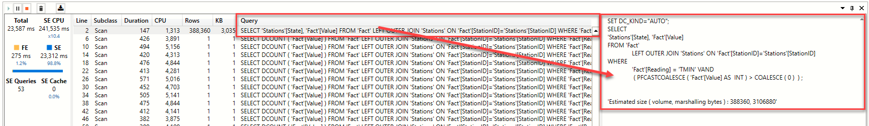
Under the “Query” column, we see the request sent to the storage engine to fulfill. The pane on the far right is a detailed view of that request. While it looks like standard T-SQL, the storage engine understands a specialized version of T-SQL, called xmSQL.
If you look at the xmSQL that is sent to the storage engine, you can see that it has optimized things so that it only brings back the two columns that I need (Fact[Value] and Stations[State]) and it has filtered the table down to minimum temperatures above zero degrees.

The rest of the storage engine queries are quicker, but there are 52 of them. What the formula engine does with the materialized table of data is that it then runs a distinct count against each set of data that matches the filter conditions, state by state! The following is a snapshot of the xmSQL generated to count how many values there are for State = South Dakota, Reading = TMIN and VALUE > 0. One query is run for each state.

There Must Be a Better Way
This seems to be a rather long-winded way to do this in less queries, right?
Think back to our performance recommendation that was mentioned earlier: filter columns, not tables. Look what happens when I identify specific columns as the filters passed to calculate as shown:
DEFINE
MEASURE Fact[PositiveValues] = CALCULATE(DISTINCTCOUNT(‘Fact'[value]), Filter(ALL(‘Fact'[Value]), ‘Fact'[Value] > 0), FILTER(ALL(‘Fact'[Reading]), ‘Fact'[Reading] = “TMIN”))
EVALUATE
CALCULATETABLE(SUMMARIZECOLUMNS(Stations[State], “Positive Values”, [PositiveValues]))

Blazing fast speeds are back! It only took one storage engine query, and that query returned the familiar 52 rows and one 1KB of data. When we pass columns as filters, the formula engine can produce a plan that is simple enough for the storage engine to process all in one query, and it doesn’t have to pass back a table, it just passes back the results. Here is the xmSQL for this query.

On a side note, there is a shorter way to write the DAX instead of explicitly calling FILTER. Here’s what that looks like:
DEFINE
MEASURE Fact[PositiveValues] = CALCULATE(DISTINCTCOUNT(‘Fact'[value]), ‘Fact'[Value] > 0, ‘Fact'[Reading] = “TMIN”)
EVALUATE
CALCULATETABLE(SUMMARIZECOLUMNS(Stations[State], “Positive Values”, [PositiveValues]))
I know there was a lot of technical content in this post, but I wanted to show some of the details of DAX code optimization.
Let’s Recap
- Filter columns, not tables
- The engine used to execute DAX queries is composed of two engines: the formula engine and the storage engine – understanding how the two operate together can help you write better DAX code
- DAX Studio captures a lot of detailed information that can help you troubleshoot why your DAX code is running slow
- This DAX stuff can get pretty complicated as the model gets larger and sometimes little changes can make a big difference
- Filter columns, not tables – it’s so important that I’ve listed it twice
As a consultant on 3Cloud’s Managed Services team, I’m passionate about optimizing and fine-tuning Power BI. When my customers can focus their attention on their business objectives and not on Power BI, I know that I’m helping make them more successful with their implementation of Power BI. If you’re interested in hearing more about how our Managed Services team can work with you to optimize your Power BI Models, DAX queries, and bring governance and order to your Power BI environment, please reach out and let us know how we can help.