Data ingestion is the process of transferring data from its source system to a data store, often a data lake. When considering your methods for data ingestion, there are many important considerations that your process must adhere to. Your data should be ingested in a timely manner, your data should arrive in its destination in an accurate format, your data should be in a format that can be transformed for analytical processes… just to name a few. Efficient data ingestion can be a daunting task depending on the complexity of your data sets. Yet, optimizing performance is a crucial part of the data ingestion process.
When you have large data sets with hundreds of millions or billions of records, ingesting that data efficiently can be a challenging feat. In many cases, these data sets may be loaded on a nightly schedule. Your nightly data ingestion pipeline must be complete within a certain time frame to avoid negatively impacting your downstream processes or analyses. So, what can you do when a job you are running each night grows too large to be processed in your time frame? How can you better manage the ingestion of these large datasets?
In a cloud-based data architecture, utilizing one server for ten hours costs the same as utilizing ten servers for one hour. Because of this, the best and most cost-effective way to optimize performance is to shorten your longest running job. An incredibly powerful way to do this is to employ a partitioning pattern. A partitioning pattern essentially involves breaking a large data ingestion job into several smaller jobs. Let’s take a few steps back and look at the overall data ingestion process to see how partitioning can fit into that process.
Ingesting Using a Partitioning Pattern
Data Ingestion to the Data Lake
A common pattern is for data to be ingested into a data lake using a data orchestration tool. A data lake is a central storage location that allows you to store vast amounts of data, both structured and unstructured. Since organization is key to maintaining your data lake, data lakes typically have several zones. Each zone fulfills a separate role or purpose in the data ingestion or transformation process. There is no single template for the number of zones or types of zones in a data lake, so these can vary across organizations depending on their needs.
For our example, our data lake includes a raw zone and a curated zone. The raw zone stores data from its source in a raw, unfiltered format. This zone also contains copies of every single version of the raw data from every single ingestion. The data from the raw zone is then transformed and loaded to the curated zone. The curated zone is more structured than the raw zone and is ready for analytical processing. Once a use case is defined, data from the curated zone can then be used to build a data warehouse.
Introducing Partitioning
So how does partitioning fit into all that? When ingesting a data source to the data lake, you can break that job into several jobs by partitioning your dataset on a selected field. Then, you can load each of the partitioned jobs to the same target in the data lake.
Let’s explore how this works using a simple sample dataset as an example.

Suppose the data above is part of a product catalog that contains millions of records. You need to ingest that data from its source system into a data lake in an efficient manner. If you follow a typical ingestion pattern, you might use the following source query to ingest your data to the data lake:
SELECT * FROM Products
This could result in a lengthy ingestion time. However, there is an alternative. Using partitioning, you can create several data ingestion jobs that pull from the source and can run in parallel and result in a faster data ingestion pipeline.
Selecting a Partitioning Field
First, you need to decide which field to partition your data on. It is most common to use dates to partition data, such as the year or month of a date. When deciding on the field to partition your data on, you must pay close attention to the cardinality of that field. A field with a high cardinality such as ProductNo, Name, or Description are not good candidates for partitioning because it could result in needing millions or billions of partitioning tasks. You could consider using low cardinality fields such as Category or Color. However, it is important to take into consideration whether that field could introduce additional values in the future. If this product catalog starts introducing new products under a new category, such as Sports or Health, this new category would need a new partitioned job in order to ingest that data. In this example, we will follow best practices of using a date field as the partitioning field. Below is an example source query for a partitioning job to ingest data to the raw zone of the data lake:
SELECT *, YEAR(LaunchDate) AS PartitionedBy
FROM Products
WHERE YEAR(LaunchDate) = 2021
You would need to create one job for each year that products were launched in order to ingest all the data. Each job should be ingested to the same target table to facilitate the consolidation of all the jobs.
Applying Partitioning to a Growing Dataset
In many cases, you won’t ingest your data from the start using partitioning. Over time, your data set will grow and eventually reach the point where it can no longer run in the necessary time frame. To implement the partitioning method, how do you handle all the data that has already been ingested in order for it to be compatible with the partitioned data?
The data that has already been ingested will need to be transformed to include a partition and a PartitionedBy column. This transformation will provide seamless integration with your incoming data.
Partitioning Existing Data
In our example, we will transform the existing data in the curated zone of the data lake using Databricks.
Let’s examine the existing data in the products table:


The first thing we need to do is to use a CTAS statement to create a new table in the curated zone of our data lake and copy our existing data to that table while adding a partition and the PartitionedBy field. We’ll name this table products_partitioned.
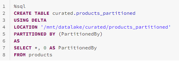
Next, let’s examine our new products_partitioned table.
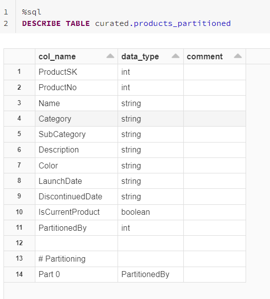


We can see that the products_partitioned table is now partitioned and has an additional PartitionedBy column. Our next step is to drop the original products table from our curated zone and remove the file from our data lake.


Repeating the Process
We could stop there and ingest all new partitioning jobs into the products_partitioned table. But in many cases, naming conventions and keeping the table name consistent is important. To get our data back into the products table, we will repeat the process.
First, we create a new table products using a CTAS statement to copy our partitioned data from products_partitioned.
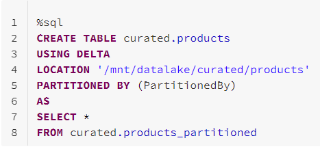
Let’s examine our newly created products table:
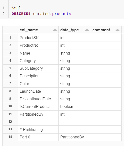


The products table is now partitioned and has a PartitionedBy field. Finally, we can clean up by dropping the products_partitioned table and removing the file from our data lake.


Bringing it all Together
Now that we have partitioned our existing data, our new partitioned jobs will begin ingesting data into this table in our data lake.
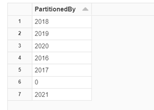
The finished product will be a partitioned table that incorporates the data that existed before the partitioning pattern was applied and efficiently ingests data partitioned by YEAR(LaunchDate).


In Conclusion
Employing a partitioning pattern is a simple, performant, and cost-effective way to resolve performance issues with data ingestion. Whether you are just beginning to build your data ingestion pipelines or you have a robust data platform but are running into issues as your data grows, partitioning can be an excellent solution to optimize performance.
Contact Us
If you’re needing help along the way, 3Cloud has a team of experts that can help you with your data platform solution needs. Contact us today!


